As we have introduced in the initial blog post, the original YOLO v3 model was pre-trained on COCO dataset with 80 dedicated classes. In this project, we will train a custom object detector for traffic signs using Google Colab as our cloud platform.
Building Darknet and Loading Pretrained Weights
The new network in YOLOv3, Darknet-53, is based on Darknet-19, which is used in YOLOv2, combining with the concept from residual networks. It includes shortcut connections with more fine-grained information, which performs as a better feature extractor. Also, it has upsampling layers merging with previous feature maps to get more meaningful information. In total, it has 106 layers to perform as a good object detector. We still use Google Colab with free GPUs as our cloud platform. We cloned the darknet from AlexeyAB’s GitHub repository, adjusted it to enable GPU, and then built the network. Since YOLOv3 has already been trained on the COCO dataset with 80 classes, we just loaded the pretrained weights from the official website so that we do not have to train the huge network from scratch and hopefully reduce the training time.
Gathering a Custom Dataset and Preparations for Training
As we have mentioned in our initial blog post, we collected images with annotations from Google’s Open Images Dataset V6 and decided to train our own detector with a new class, which is traffic signs. Every single image comes with a .txt file annotating coordinates of the boundary, the height and the width of the object. The figure below is obtained from AlexeyAB’s GitHub repository which explains the annotation for the training set.
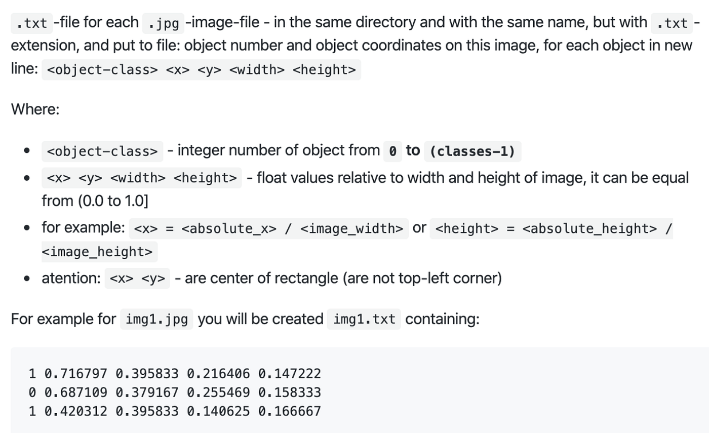 An Example of Annotation
Source: AlexeyAB’s GitHub repository
We copied over the configuration file of YOLOv3 and made some modifications according to our new single class detector. We made the maximum number of batches to be 2000 per class, which should be 2000 in this case. The number of steps are respectively 80% and 90% percent of the number of batches to make sure it iterates enough, thus we have 1600 and 1800 for steps. Since YOLOv3 predicts bounding boxes at 3 different scales, the last of convolutional layers of every feature extractor block predicts a 3-d tensor encoding bounding box, objectness, and class predictions. In total, the tensor is N * N * ((4+1+1) * 3) for the 4 bounding box offsets (manifested in annotations), 1 objectness detection (confidence level), and 1 class prediction. Thus the number of filters, which is the same as the number of feature maps, is 18 in this case. Before running the config files, the number of classes is set to one for each of the 3 yolo layers performing bounding box prediction, while the number of filters should be 18 for each convolutional layer before it.
To determine the bounding box anchors (also called priors), YOLOv3 still uses k-means clustering. The initial training will be more stable if we start with diverse guesses of the shapes of bounding boxes that are common for real-life objects. In this case, we just chose 9 clusters which are shown as anchors and 3 scales arbitrarily and then divided them evenly across scales. Here are the parameters of one of the yolo layers and one convolutional layer above it in the configuration file. It also shows the width and height of the 9 anchors.
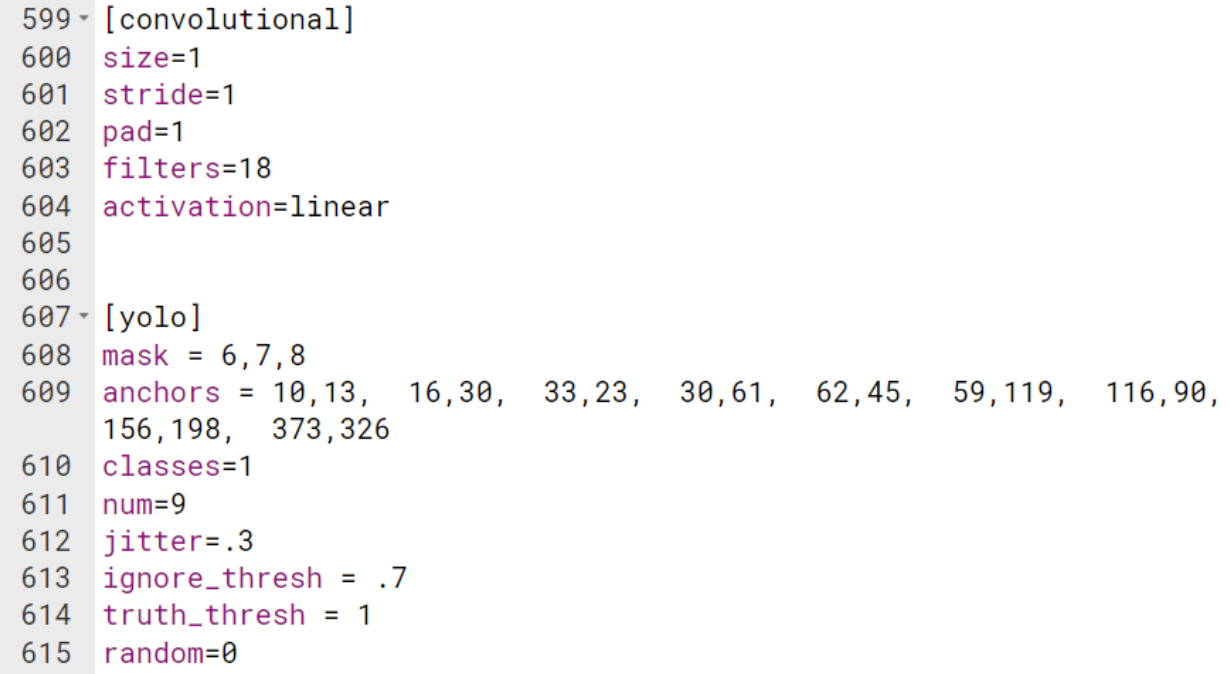
Parameters of Hidden Layers
Besides, obj.names and obj.data should be modified based on the target class(es) we want to train. In this case, we would include one class name as “traffic sign” and set up the number of classes as one in the obj.data file.
Considering there might be automatic interruption in Colab, we would like to take advantage of the backup folder specified in the obj.data file. The program would save current weights in the backup folder after training about every other 40 images.
Training the Custom Object Detector
With all the previous preparations, we are ready to train the detector. Our training dataset has over 2818 images of traffic signs, and it takes about 4–6 hours to train the customized detector. Here is a plot showing the loss through the training process:
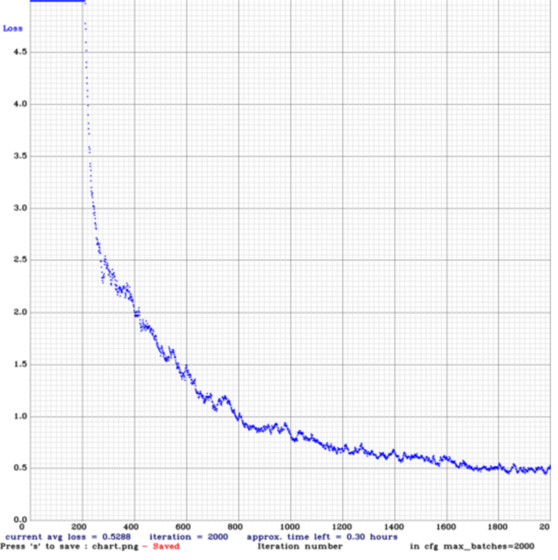 Loss Curve in the Training Process
YOLO uses sum-squared error between the predictions and the ground truth to calculate loss and it consists of the classification loss, the localization loss (errors between the predicted boundary box and the ground truth) and the confidence loss (the objectness of the box).
We can see that over 400 iterations, the average loss has been reduced to lower than 2, which indicates an accurate model. In the end, the average loss is lower than 0.5.
Although the original YOLOv3 is able to detect stop signs, it is unable to detect traffic signs other than stop signs since they are not in the 80 classes it has been trained. Now we are happy to see traffic signs can be detected with our own detector!
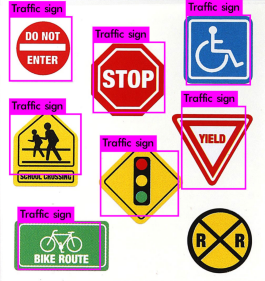 Detection Result
Source: Google Image
References
This great GitHub repo provides the implementation of several pre-trained models and illustrates how to train a custom detector. We basically followed this step-by-step tutorial to build our network.
This is the document of weights of YOLOv3 pre-trained on COCO dataset. We used it to reduce our training time.
Real-time Object Detection with YOLO, YOLOv2 and now YOLOv3
This great Medium post clearly explains the details of YOLO from its original papers including the structure of the network and the improvement from YOLO to YOLOv3. The illustration of loss function and bounding box are explicit and work as a good supplementation for the paper.